Showing posts with label images. Show all posts

Tuesday, 16 March 2010

Fractals with Octave: The Whole Shebang

After all this time writing this simple series of how to create fractals with Octave, I finally got to the end of it and published the code on GitHub so here is a nifty summary.

Articles

Each article has a link to the previous and following ones so you can just start with the first one and follow up to the last one.

Code

The code is available on GitHub and can be downloaded from the project page, where you will also find some installation instructions.

If you're interested, please download the code and if you use it to create stunning images, I'd love to hear from you. If you think you can improve the code, don't hesitate to suggest changes or fork it.

References

To quote the project page, none of this was created in a vaccum. I used a number of offline and online references so if you are interested in the subject of fractals, you could do a lot worse than checking them out:

Saturday, 27 February 2010

Fractals with Octave: Original Function Studied by Gaston Julia

The story so far

After another long pause, here is the sixth instalment of this series on fractals with Octave. In this article, we have a look at the complex series that started is all, the one that Gaston Julia was interested in.

Once Upon A Time: The Original Fractal Function

The classic Mandelbrot set we all know and love is derived from quite a simple series, described in the very first article of this series. Gaston Julia was interested in a slightly more complex series, as explained by Paul Bourke:

zn+1=z4 + z3/(z-1) + z2/(z3+4z2+5) + c

The initial condition is:

z0=0

The Mandelbrot Set

We can produce a Mandelbrot set of that equation with the mandelbrot function that we created in previous articles.

octave:1> Mj=mandelbrot(-1.4+1.05i,1.4-1.05i,320,64,
> @(z,c) z.^4.+z.^3./(z-1)+z.^2./(z.^3.+4*z.^2.+5).+c;
octave:2> imagesc(Mj)

And here is the result:

Original Julia Series, Mandelbrot Set

We can then zoom on the bottom right corner of that image.

octave:1> Mjz=mandelbrot(0.25-0.65i,0.45-0.8i,320,64,
> @(z,c) z.^4.+z.^3./(z-1)+z.^2./(z.^3.+4*z.^2.+5).+c;
octave:2> imagesc(Mjz)

Original Julia Series, Mandelbrot Set x10

And again.

octave:1> Mjzz=mandelbrot(0.378-0.725i,0.398-0.74i,320,64,
> @(z,c) z.^4.+z.^3./(z-1)+z.^2./(z.^3.+4*z.^2.+5).+c;
octave:2> imagesc(Mjzz)

Original Julia Series, Mandelbrot Set x100

And again!

octave:1> Mjzzz=mandelbrot(0.3863-0.7314i,0.3883-0.7329i,320,64,
> @(z,c) z.^4.+z.^3./(z-1)+z.^2./(z.^3.+4*z.^2.+5).+c;
octave:2> imagesc(Mjzzz)

Original Julia Series, Mandelbrot Set x1000

The Julia Set

Now, let's have a look at the Julia set for the same series and for c=0.3873-0.7314i, which is the point towards which we zoomed on in the Mandelbrot set.

octave:1> Jj=julia(-1.2+1.6i,1.2-1.6i,240,64,0.3873-0.7314i,
> @(z,c) z.^4.+z.^3./(z-1)+z.^2./(z.^3.+4*z.^2.+5).+c;
octave:2> imagesc(Jj)

Original Julia Set, c=0.3873-0.7314i

Let's zoom into that picture.

octave:1> Jjz=julia(0.2+0.1i,0.4-0.05i,320,64,0.3873-0.7314i,
> @(z,c) z.^4.+z.^3./(z-1)+z.^2./(z.^3.+4*z.^2.+5).+c;
octave:2> imagesc(Jjz)

Original Julia Set, c=0.3873-0.7314i, x10

And again.

octave:1> Jjzz=julia(0.366+0.09i,0.386+0.075i,320,64,0.3873-0.7314i,
> @(z,c) z.^4.+z.^3./(z-1)+z.^2./(z.^3.+4*z.^2.+5).+c;
octave:2> imagesc(Jjzz)

Original Julia Set, c=0.3873-0.7314i, x100

And again!

octave:1> Jjzzz=julia(0.366+0.09i,0.386+0.075i,320,64,0.3873-0.7314i,
> @(z,c) z.^4.+z.^3./(z-1)+z.^2./(z.^3.+4*z.^2.+5).+c;
octave:2> imagesc(Jjzzz)

Original Julia Set, c=0.3873-0.7314i, x1000

The End

This is the last article in this series. I hope you've enjoyed it, even if it took me a very long time to finish it. Have a play with the Octave functions described throughout the articles, modify them, improve them, there's a lot of fun stuff to do and amazing pictures to create with fractals.

Wednesday, 26 August 2009

Fractals with Octave: Burning Ship

The story so far

After a long pause, here is the fifth instalment of this series on fractals with Octave. This time I will look at a fractal called the Burning Ship because of its output that looks like a ship going up in flames.

Burning Ship

The fractal is a Mandelbrot set that has a generating series defined by:

zn+1=(|Re(zn)|+i|Im(zn)|)2+c

where the Re and Im are the functions that return the real and imaginary parts of a complex number. The initial condition is:

z0=0

This fractal can be directly produced with the mandelbrot function we created in previous articles. In addition, we will take r=200 as a divergence limit.

octave-3.0.1:1> Mbs=mandelbrot(-2.5-2i,1.5+i,320,64,
> @(z,c) (abs(real(z))+i*abs(imag(z))).^2.+c,200);
octave-3.0.1:2> imagesc(Mbs)

Octave should open the Gnuplot window and display an image similar to this:

Burning Ship

Burning Ship fractal

Now let's zoom on this fractal centre left by a factor of 30:

octave-3.0.1:1> Mbsz=mandelbrot(-1.8-0.06i,-1.7+0.02i,320,64,
> @(z,c) (abs(real(z))+i*abs(imag(z))).^2.+c,200);
octave-3.0.1:2> imagesc(Mbsz)

Octave should open the Gnuplot window and display an image similar to this:

Burning Ship, left centre zoom x30

Burning Ship, centre left zoom x30

As usual with a fractal like this, the zoomed image looks very similar to the original. Now let's have a look at a related fractal called the Bird of Prey.

Bird of Prey

In the same way that you can produce interesting variations on the classic Mandelbrot set by changing the power used in the series, we can do the same with the Burning Ship series. So let's increase the power in the series above from 2 to 3:

zn+1=(|Re(zn)|+i|Im(zn)|)3+c

This cubic series produces a fractal called the Bird of Prey.

octave-3.0.1:1> Mbs3=mandelbrot(-1.5-1.5i,1.5+1.5i,320,64,
> @(z,c) (abs(real(z))+i*abs(imag(z))).^3.+c,200);
octave-3.0.1:2> imagesc(Mbs3)

You'll note that I chose the boundary values for the complex plane so that I would get a square image centered on the origin. Here is the resulting image:

Bird of Prey

Bird of Prey

Next

That's it for the Burning Ship. Next in this series, we will look at the original fractal that Gaston Julia was interested in.

Tuesday, 26 May 2009

Fractals with Octave: Trigonometric and Exponential Functions

The story so far

In this fourth instalment of this series on fractals with Octave, I'll have a look at the Mandelbrot and Julia sets generated by non-polynomial series. Polynomials are fine but they can be a bit boring so what about introducing a sine or exponential in the mix? The original idea for this came from an excellent set of articles and examples by Paul Bourke.

Sine function

The first series we will use is defined thus:

zn+1=c sin(zn)

That's simple enough and very easy to code in Octave so as our mandelbrot and julia functions now have the ability to take a generating series as argument, it should be no problem. But before doing that, we need to know what value to give to r so that we know when the series diverges and when we can stop iterating. In the very first article, we saw that:

[...] for a given polynomial series, there exists a value r such that if for any n, |zn|>r, then the series diverges.

This only applies to polynomials. The series above is not a polynomial series and its condition for divergence is that the imaginary part of zn be greater than 50. That doesn't work well with our current code that expects a simple integer. We could replace the integer parameter expected by the mandelbrot and julia functions with a function handle but that would make their usage more complex when using polynomial series. Luckily, we can have the best of both worlds because Octave uses a weakly typed language: the type of a parameter passed to a function is not specified in the function definition, meaning that you can pass anything, you just have to hope that it is what the function expects. While this can be seen as a drawback for long and complex programs where validation can be cumbersome, it is actually a useful feature for a high level language like Octave where functions tend to be short. To make it work, we need to modify the mjcore function so that it can accept a function handle or an integer as its fifth parameter and act accordingly. For this, we will use the Octave isa built-in function to identify whether the parameter is a function handle. Here's how to modify the mjcore function:

mjcore.m

function M=mjcore(z,c,niter,f,r)
  if(isa(r,"function_handle"))
    rf=r;
  else
    rf=@(z) abs(z)<r;
  endif
  M=zeros(length(z(:,1)),length(z(1,:)));
  for s=1:niter
    mask=abs(z)<rrf(z);
    M(mask)=M(mask)+1;
    z(mask)=f(z(mask),c(mask));
  endfor
  M(mask)=0;
endfunction

That's all great and now we should be able to create our first sine Mandelbrot. We need to make sure that we reverse the comparison operator in the last parameter because our code is built so that we provide a convergence condition rather than a divergence one:

octave-3.0.1:1> Msin=mandelbrot(-1.2*pi+0.9*pi*i,1.2*pi-0.9*pi*i,
> 320,64,
> @(z,c) c.*sin(z), @(z) abs(imag(z))<=50);
octave-3.0.1:2> imagesc(Msin)

And we end up with... a dark blue rectangle, not quite what was expected. This is because in this form, the value of z0 is 0, therefore sin(z0) is also 0 and so is c sin(z0): the series is always null and never diverges. To correct this, we would need to have z0=c, that is initialise the series to the values of c. But if we do that in the code of the mandelbrot function, it will break some of our previous examples. That is unless we can specify a special value of z0 to the mandelbrot function to force it to initialise to z0=c. A similar trick to what we did for r above can do that: if the given parameter is the special string "c", initialise to c, otherwise assume the parameter is an integer and initialise as before. Here is the modified mandelbrot function:

mandelbrot.m

function M=mandelbrot(cmin,cmax,hpx,niter,
                      f=@(z,c) z.^2.+c,r=2,
                      z0=0)
  vpx=round(hpx*abs(imag(cmax-cmin)/real(cmax-cmin)));
  z=zeros(vpx,hpx).+z0;
  [cRe,cIm]=meshgrid(linspace(real(cmin),real(cmax),hpx),
                     linspace(imag(cmin),imag(cmax),vpx));
  c=cRe+i*cIm;
  if(strcmp("c",z0))
    z=c;
  else
    z=zeros(vpx,hpx).+z0;
  endif
  M=mjcore(z,c,niter,f,r);
endfunction

After that modification, we can run the mandelbrot function again with our new special parameter:

octave-3.0.1:1> Msin=mandelbrot(-1.2*pi+0.9*pi*i,1.2*pi-0.9*pi*i,
> 320,64,
> @(z,c) c.*sin(z), @(z) abs(imag(z))<=50, "c");
octave-3.0.1:2> imagesc(Msin)

Octave should open the Gnuplot window and display an image similar to this:

Sine Mandelbrot Set

Sine Mandelbrot Set

We can also generate a sine Julia set without any change to the julia function:

octave-3.0.1:1> Jsin=julia(-2.4*pi+1.8*pi*i,2.4*pi-1.8*pi*i,
> 320,64,1+0.5i,
> @(z,c) c.*sin(z), @(z) abs(imag(z))<=50);
octave-3.0.1:2> imagesc(Jsin)

Sine Julia Set

Sine Julia Set

Cool stuff! So let's have a look at other non-polynomial functions and their output.

Cosine

This series is defined by:

zn+1=i c cos(zn)

And has the same convergence condition than the previous series.

octave-3.0.1:1> Mcos=mandelbrot(-1.2*pi+0.9*pi*i,1.2*pi-0.9*pi*i,
> 320,64,
> @(z,c) i.*c.*cos(z), @(z) abs(imag(z))<=50, "c");
octave-3.0.1:2> imagesc(Mcos)

Cosine Mandelbrot Set

Cosine Mandelbrot Set
octave-3.0.1:1> Jcos=julia(-2.4*pi+1.8*pi*i,2.4*pi-1.8*pi*i,
> 320,64,0.55+1.195i,
> @(z,c) i.*c.*cos(z), @(z) abs(imag(z))<=50);
octave-3.0.1:2> imagesc(Jcos)

Cosine Julia Set

Cosine Julia Set

Tangent

This series is defined by:

zn+1=c tan(zn)

And uses the same convergence function as a polynomial with the default value of r.

octave-3.0.1:1> Mtan=mandelbrot(-1.4+1.4i,1.4-1.4i,
> 320,64,
> @(z,c) c.*tan(z), :, "c");
octave-3.0.1:2> imagesc(Mtan)

Tangent Mandelbrot Set

Tangent Mandelbrot Set
octave-3.0.1:1> Jtan=julia(-1.4+1.4i,1.4-1.4i,
> 320,64,(1+i)*sqrt(2)/2,
> @(z,c) c.*tan(z));
octave-3.0.1:2> imagesc(Jtan)

Tangent Julia Set

Tangent Julia Set

Exponential

First, let's multiply the exponential using the following series:

zn+1=c exp(zn2)

This series uses the default values for r and z0.

octave-3.0.1:1> Mexp1=mandelbrot(-1.4+2i,1.4-2i,
> 240,64,
> @(z,c) c.*exp(z.^2));
octave-3.0.1:2> imagesc(Mexp1)

Exponential Mandelbrot Set #1

Exponential Mandelbrot Set #1

Then, let's add to the exponential using the following series:

zn+1=exp(zn2)+c

This series also uses the default values for r and z0.

octave-3.0.1:1> Mexp2=mandelbrot(-2.2+2i,1-2i,
> 240,64,
> @(z,c) exp(z.^2).+c);
octave-3.0.1:2> imagesc(Mexp2)

Exponential Mandelbrot Set #2

Exponential Mandelbrot Set #2

Cactus

Finally, let's draw a cactus using the following series:

zn+1=zn3+(z0-1)zn-z0

This series uses the default values for r and the special value z0=c.

octave-3.0.1:1> Mcactus=mandelbrot(-0.8+0.6i,0.8-0.6i,
> 320,64,
> @(z,c) z.^3.+(c.-1).*z.-c,:,"c");
octave-3.0.1:2> imagesc(Mcactus)

Cactus Mandelbrot Set

Cactus Mandelbrot

Next

Next in this series, we will look at a fractal called the Burning Ship.

Friday, 27 March 2009

Fractals with Octave: Other Polynomials

The story so far

In the third instalment of this series on fractals with Octave, I want to change the polynomial series used to generate the Mandelbrot and Julia sets. So far, I've used the classic series, defined by:

zn+1=zn2+c

In the previous articles, I showed what happened when you varied the initial values for z0 and c but why not go further and use a different polynomial altogether?

Code review

Before jumping into the thick of it, let's have a look at the code produced so far. We created 4 functions:

function M=mjcore(z,c,niter)
The core function shared by the mandelbrot and julia functions;
function M=mandelbrot(cmin,cmax,hpx,niter)
The function that produces a colour map image as per the Mandelbrot algorithm;
function M=mandelbrotz0(cmin,cmax,hpx,niter,z0)
A variation of the mandelbrot function that takes an extra argument in order to specify an initial z0 value;
function M=julia(zmin,zmax,hpx,niter,c)
The function that produces a colour map image as per the Julia algorithm.

There is very little difference between the mandelbrot and mandelbrotz0 functions: mandelbrot just uses a default value of 0 for z0. In fact, we could merge both functions into one using the default argument construct supported by Octave. Here's a new version of the mandelbrot.m file that uses it:

mandelbrot.m

function M=mandelbrot(cmin,cmax,hpx,niter,z0=0)
  vpx=round(hpx*abs(imag(cmax-cmin)/real(cmax-cmin)));
  z=zeros(vpx,hpx).+z0;
  [cRe,cIm]=meshgrid(linspace(real(cmin),real(cmax),hpx),
                     linspace(imag(cmin),imag(cmax),vpx));
  c=cRe+i*cIm;
  M=mjcore(z,c,niter);
endfunction

Having done this, we can now create the classic Mandelbrot image as we did previously, using four arguments:

octave-3.0.1:1> Mc=mandelbrot(-2.1+1.05i,0.7-1.05i,640,64);

Create the Mandelbrot image with z0=0.2+0.2i by adding a fifth argument:

octave-3.0.1:2> Mz0=mandelbrot(-2.1+1.05i,0.7-1.05i,640,64,0.2+0.2i);

And we can delete the mandelbrotz0.m file. Note that you could also explicitly tell Octave to use the default for the fifth argument by specifying a colon (:) in its place, so you could produce the classic Mandelbrot this way:

octave-3.0.1:3> Mc=mandelbrot(-2.1+1.05i,0.7-1.05i,640,64,:);

This is not very useful in this context but we will see a use for it later.

Function handles and anonymous functions

In order to be able to change the polynomial used to calculate the fractal image, we need to be able to specify to the mjcore function what function to use when calculating the series. We could create a whole library of mjcore derivatives but that would quickly get tedious. Instead, we can use Octave's function handles. A function handle is a fancy way to say that in Octave, any variable can be a function. Therefore, we can just pass the function as an argument of the mjcore function. And while we're at it, we'll also pass r as an argument because, as we saw in the first article, the value for r is dependant on the function used in the series. So here is a modified version of that function:

mjcore.m

function M=mjcore(z,c,niter,f,r)
  M=zeros(length(z(:,1)),length(z(1,:)));
  for s=1:niter
    mask=abs(z)<r;
    M(mask)=M(mask)+1;
    z(mask)=f(z(mask),c(mask));
  endfor
  M(mask)=0;
endfunction

That's all good and well but we've just moved the problem further into the mandelbrot and julia functions: those functions will have to specify parameters accordingly and use sensible defaults so that if we omit the values for f and r, it will calculate the classic sets using the series zn+1=zn2+c (i.e. the function f=z2+c) and r=2. To do that, we are going to use the default argument construct explained above and combine it with an anonymous function. Using anonymous functions, we can define a variable f that is a handle on a function that implements the classic algorithm:

octave-3.0.1:4> f=@(z,c) z.^2.+c;

As shown above, we can use exactly the same syntax to specify default arguments to the mandelbrot and julia functions. Here are the new versions of those two functions:

mandelbrot.m

function M=mandelbrot(cmin,cmax,hpx,niter,
                      f=@(z,c) z.^2.+c,r=2,
                      z0=0)
  vpx=round(hpx*abs(imag(cmax-cmin)/real(cmax-cmin)));
  z=zeros(vpx,hpx).+z0;
  [cRe,cIm]=meshgrid(linspace(real(cmin),real(cmax),hpx),
                     linspace(imag(cmin),imag(cmax),vpx));
  c=cRe+i*cIm;
  M=mjcore(z,c,niter,f,r);
endfunction

julia.m

function M=julia(zmin,zmax,hpx,niter,c,
                 f=@(z,c) z.^2.+c,r=2
                 )
  vpx=round(hpx*abs(imag(zmax-zmin)/real(zmax-zmin)));
  [zRe,zIm]=meshgrid(linspace(real(zmin),real(zmax),hpx),
                     linspace(imag(zmin),imag(zmax),vpx));
  z=zRe+i*zIm;
  cc=zeros(vpx,hpx)+c;
  M=mjcore(z,cc,niter,f,r);
endfunction

Cubic sets

We can now produce cubic Mandelbrot and Julia sets by setting the power to 3 instead of 2:

octave-3.0.1:5> Mn3=mandelbrot(-1.2+1.6i,1.2-1.6i,240,64,
> @(z,c) z.^3.+c);
octave-3.0.1:6> imagesc(Mn3)

Cubic Mandelbrot Set

Cubic Mandelbrot image
octave-3.0.1:7> Jn3=julia(-1.6+1.2i,1.6-1.2i,320,64,0.4,
> @(z,c) z.^3.+c);
octave-3.0.1:8> imagesc(Jn3)

Cubic Julia Set for c=0.4

Cubic Julia image for c=0.4

Quartic sets

Increasing the power to 4, we get quartic sets:

octave-3.0.1:9> Mn4=mandelbrot(-1.2+1.6i,1.2-1.6i,320,64,
> @(z,c) z.^4.+c);
octave-3.0.1:10> imagesc(Mn4)

Quartic Mandelbrot Set

Quartic Mandelbrot set
octave-3.0.1:11> Jn4=julia(-1.6+1.2i,1.6-1.2i,320,64,-1,
> @(z,c) z.^4.+c);
octave-3.0.1:12> imagesc(Jn4)

Quartic Julia Set for c=-1

Quartic Julia set for c=-1

Note that for a series defined by the equation zn+1=znp+c, the resulting Mandelbrot set will show p-1 secondary "blobs" while the Julia set will show p secondary "blobs".

Decimal power

The power doesn't have to be an integer. Using a decimal value, such as 2.5, generates the following Mandelbrot image, that is halfway between the normal and cubic sets:

octave-3.0.1:13> Mn2_5=mandelbrot(-1.6+1.2i,1.6-1.2i,320,64,
> @(z,c) z.^2.5.+c);
octave-3.0.1:14> imagesc(Mn2_5)

Mandelbrot Set for p=2.5

Mandelbrot set for p=2.5

Complex power

Using a complex power, such as 2+0.1i, generates a skewed set:

octave-3.0.1:15> Mn2_01i=mandelbrot(-2.2+1.2i,1.0-1.2i,320,64,
> @(z,c) z.^(2+.1i).+c);
octave-3.0.1:16> imagesc(Mn2_01i)

Mandelbrot Set for p=2+0.1i

Mandelbrot set for p=2+0.1i

More complex polynomial

Using a series based on a more complex polynomial, such as zn+1=zn2+zn+c, generates the following set:

octave-3.0.1:17> Mp=mandelbrot(-2+1.05i,0.8-1.05i,320,64,
> @(z,c) z.^2.+z.+c);
octave-3.0.1:18> imagesc(Mp)

Mandelbrot Set for series zn+1=zn2+zn+c

Mandelbrot set for series zn+1=zn^2+zn+c

Bootnote

Having modified the mandelbrot function to include the f and r arguments before the z0 argument, we now need to use the colon argument for f and r to produce a classic Mandelbrot with a different value of z0:

octave-3.0.1:2> Mz0=mandelbrot(-2.1+1.05i,0.7-1.05i,640,64,:,:,0.2+0.2i);

I could have left the z0 argument in fifth position to avoid having to do this but I felt that the f and r arguments were more likely to be provided so are better specified first in the function's signature.

Next

In the next article in this series, Trigonometric and Exponential Functions, we'll look at non-polynomial series.

Tuesday, 17 February 2009

Fractals with Octave: More on the Classic Sets

The story so far

In the second instalment of this series on fractals with Octave, I will generate more images by changing some of the parameters of the different functions presented in the first article. But before doing that, I'll briefly explain how to save the generated images and say a word on colour maps.

Saving images

The images that the functions described in the previous post generate are colour mapped images. Each element of a result matrix is an integer value that corresponds to a colour index. Octave has a very easy way to save that type of images using the well named saveimage function. To save the images generated, we just need to do:

octave:1> saveimage(file name, matrix, type, colour map);

The file name parameter is the name of the image file we want to save the image to. Give it a .ppm extension, we'll see why in a second. The matrix parameter is the matrix generated by the mandelbrot or julia functions presented in the previous article. The type parameter is the type of the image: we will use the PPM type as it is supported natively by Octave so that attribute should just be ppm. The colour map attribute is a colour map to use in the file. Octave has a default colour map that contains 64 colours from dark blue to light blue, then from yellow to red and white, similar to a contour map. It can be invoked by the colormap command. Putting all this together, creating a classic Mandelbrot image and saving it can be done this way:

octave:1> M=mandelbrot(-2.1+1.05i,0.7-1.05i,320,64);
octave:2> saveimage("mandelbrot.ppm", M, "ppm", colormap);

The PPM file format is understood natively by Linux but if you want to transform it into a more widely used format such as GIF or PNG, you can use ImageMagick or The GIMP. Avoid the JPEG format as it's not well suited to that type of computer generated images.

That's all well and good but what if you want your generated images to use a different colour map from the default? Let's create one. Octave understands a colour as a row vector that has 3 elements corresponding to the red, green and blue components of a colour. Each element is a real value between 0.0 and 1.0. So for example bright red would be [1, 0, 0] and 50% grey would be [0.5, 0.5, 0.5]. A colour map is a 3 column matrix where each row in the column is a colour. As an example, the following is a 5 colour map that defines a gradient from bright red to bright green:

   1.00000   0.00000   0.00000
   0.75000   0.25000   0.00000
   0.50000   0.50000   0.00000
   0.25000   0.75000   0.00000
   0.00000   1.00000   0.00000

We can build such a gradient by using the linspace command to evenly spread values. We will need to do that for each red, green and blue component and then combine all three with the cat command. Each vector produced by linspace will represent a column in the colour map matrix. However linspace produces row vectors so we need to transpose them before concatenating them using the ' operator. The following will produce a 64 value gradient from dark blue to white:

mycolmap=cat(2,
linspace(0, 1, 64)',
linspace(0.2, 1, 64)'
);

The resulting colour map can then be used to save the image. Note that for best results, the number of colours in the colour map should be the same as the number of iterations used when producing the fractal image.

Zooming into the Mandelbrot set

With the preamble out of the way, let's create some more fractal images. You can now save them for posterity! Some great images can be obtained by zooming somewhere on the edges of the Mandelbrot set. Let's zoom to the top centre of the set:

octave:1> Mcz=mandelbrot(-0.27+i,0.05+0.76i,320,64);
octave:1> imagesc(Mcz)

Octave should open the Gnuplot window and display the following image:

Mandelbrot Set, Top Centre Zoom

Zoom onto the top centre edge of the Mandelbrot set

This image shows a number of artefacts that are similar to the complete set. Zooming further on those would show them in more details. And as this is a fractal set, you can zoom as much as you want and discover more interesting structures.

Mandelbrot with a non-null z0

In the first article, we built the mandelbrot function based on the assumption that the initial value of the zn series, z0, was 0 for all values of c. It doesn't have to be. So let's create a modified mandelbrot function that can set a different value for z0 and call it mandelbrotz0. Copy the mandebrot.m file described in the previous article into a mandelbrotz0.m and modify it accordingly:

mandelbrotz0.m

function M=mandelbrotz0(cmin,cmax,hpx,niter,z0)
  vpx=round(hpx*abs(imag(cmax-cmin)/real(cmax-cmin)));
  z=zeros(vpx,hpx).+z0;
  [cRe,cIm]=meshgrid(linspace(real(cmin),real(cmax),hpx),
                     linspace(imag(cmin),imag(cmax),vpx));
  c=cRe+i*cIm;
  M=mjcore(z,c,niter);
endfunction

Then, let's run this function with z0=0.2+0.2i:

octave:1> Mz0=mandelbrotz0(-2.1+1.05i,0.7-1.05i,320,64,0.2+0.2i);
octave:2> imagesc(Mz0)

Octave should refresh the Gnuplot window and display the following image:

Mandelbrot Set, z0=0.2+0.2i

Mandelbrot set with z0=0.2+0.2i

Quirky! It's as if the Mandelbrot set was exploding like a ruptured balloon! Other values produce interesting results and the further they are from 0, the more distorted the set is.

Zooming into the Julia set

After the experiments with the Mandelbrot set above, let's explore the Julia set a bit more than we did last time, using c=-0.1+0.9i. Let's calculate the whole set for this value:

octave:1> Jc2=julia(-1.6+1.2i,1.6-1.2i,320,64,-0.1+0.9i);
octave:2> imagesc(Jc2)

Which produces the following image:

Julia Set, c=-0.1+0.9i

Julia set, c=-0.1+0.9i

Then, let's zoom 10 times to a point slightly off centre:

octave:1> Jc2z=julia(-0.16+0.24i,0.16,320,64,-0.1+0.9i);
octave:2> imagesc(Jc2z)

Julia Set, c=-0.1+0.9i, zoom x10

Julia set, c=-0.1+0.9i, zoom x10

And again:

octave:1> Jc2zz=julia(-0.016+0.072i,0.016+0.048i,320,64,-0.1+0.9i);
octave:2> imagesc(Jc2zz)

Julia Set, c=-0.1+0.9i, zoom x100

Julia set, c=-0.1+0.9i, zoom x100

Cool pictures, don't you think?

Bootnote

Having created a slightly more generic mandelbrotz0 function above, we can now re-write and simplify the original mandelbrot function by calling mandelbrotz0:

mandelbrot.m

function M=mandelbrot(cmin,cmax,hpx,niter)
  M=mandelbrotz0(cmin,cmax,hpx,niter,0);
endfunction

Next

In the next article of this series, Other Polynomials, we look at what happens when we use a different complex series than the standard one.

Friday, 19 December 2008

Fractals with Octave: Classic Mandelbrot and Julia

After reading this article in FSM, I decided to have a go at doing fractal images with Octave. In the process, I discovered quite a bit about fractals so here is the result of those experiments. First I'll build some classic Mandelbrot and Julia fractal images.

Pre-Requisites

All the code below was created on Ubuntu using Octave. If you don't use Ubuntu, check with your distribution or follow the instructions on the Octave web site. If you have Ubuntu, you just need to install the Octave package. To do this, open a terminal and type the following at the command line:

$ sudo apt-get install octave

Alternatively, considering that Octave is meant to be compatible with MATLAB, it should be possible to adapt everything in this series to MATLAB.

Fractal Basics

Fractals is a term that encompasses a variety of mathematical constructions that all have a property in common: they are inherently recursive. This means that you can only ever produce an approximation of a fractal to a given level of precision, which is why their study is well adapted to computational approximation methods, what a computer is inherently designed for.

Mandelbrot and Julia sets are generated as a result of studying the convergence properties of series in the complex plane. The series that is most commonly used is:

zn+1=zn2+c

This series converges or diverges for large values of n, depending on the value of z0 and c. All well and good but how does that help us produce cool fractal images with Octave? We're getting there.

The Julia and Mandelbrot sets

The Julia sets (from Gaston Julia who first studied such series) show the behaviour of complex series when you vary the value of z0 in the complex plane, for a given value of c. But the question is then: what are interesting values of c?

Conversely, the Mandelbrot sets (from Benoît Mandelbrot who first used a computer to study such series) show the behaviour of the same series when you vary the value of c in the complex plane, for a given value of z0, the most classic example using z0=0.

Constructing an Image

So, if we map the pixels of our image to the complex plane, we can associate a value of c to each pixel and calculates values of zn for z0=0 in order to obtain a Mandelbrot image.

But what values of n are we interested in and what do we do with the value we calculate? As said above, we are interested in whether the series diverges or not so we could colour a pixel in white if it diverges and in black if it converges.

How do we know whether the series converges or diverges then? Some people much smarter than I am have proven that for a given polynomial series, there exists a value r such that if for any n, |zn|>r, then the series diverges. For the polynomial given above, r=2.

So now, we can identify for each point whether the series diverges or converges so we can colour the corresponding pixel white or black. But most Mandelbrot images you see in the wild are not black and white, they are rather colourful: so how do they get all their funky colours? Each colour is associated with how quickly the series diverges. To obtain that effect, we will associate the value 0 with points that converge and a number greater than 0 for points that diverge. That number will be the lowest value of n for which |zn|>r. Each value will then be associated to a colour in a colour to produce the final image.

The Code

After all this background, it's time to do some coding. But first, we need to ensure that Octave knows where to find the functions we will define. The way Octave works, it looks for function files in its path and expects each function to be stored in a file of the same name with the .m suffix. By default, the Octave path doesn't include any directory for which you have write access so what I did was to create an octave directory in my home directory as well as a .octaverc file that adds ~/octave to the path:

.octaverc

addpath("~/octave");

From now on, every .m file in the ~/octave directory will be found by Octave and recognised as a function file. You will need to restart Octave for this to take effect.

Now that the preamble is out of the way, we can start coding in earnest so let's fire a trusty file editor and create a file called mandelbrot.m in the ~/octave directory. In this file, we are going to define a mandelbrot function that takes 4 arguments: cmin, cmax, hpx and niter, corresponding respectively to the minimum and maximum values of c, the number of horizontal pixels in the image and the number of iterations:

function M=mandelbrot(cmin,cmax,hpx,niter)

The aim of this function will be to populate the matrix M with the colour values of pixels. The first thing we do is calculate the vertical number of pixels such that ratio of the final picture is the same as the one given implicitly by cmin and cmax:

vpx=round(hpx*abs(imag(cmax-cmin)/real(cmax-cmin)));

We then initialise z, c and M. z and M are easy as they just need to be initialised to zeroes. However, note that the vertical dimension is the first one because Octave orders a matrix per columns first. c is a bit more complicated as it need to be initialised to a matrix that is vpx by hpx in size with real values spread along the horizontal axis and imaginary values spread along the vertical axis. The linspace function produces a vector of values evenly spread between the minimum and maximum across the given number of points. The meshgrid function then produces 2 real matrices out of those 2 vectors that are then merged together as a complex matrix.

z=zeros(vpx,hpx);
[cRe,cIm]=meshgrid(linspace(real(cmin),real(cmax),hpx),
                   linspace(imag(cmin),imag(cmax),vpx));
c=cRe+i*cIm;
M=zeros(vpx,hpx);

The final part of the function is the main loop. Here we use Octave's full potential using matrix calculation and a matrix mask. The mask is calculated so that it contains all the points that have not yet diverged and the corresponding entries in the result matrix are incremented. Points that diverge are not incremented and are excluded from the next calculation. Finally, we set the remaining points, that is the ones that haven't diverged after niter iterations, to 0.

for s=1:niter
  mask=abs(z)<2;
  M(mask)=M(mask)+1;
  z(mask)=z(mask).^2+c(mask);
endfor
M(mask)=0;

Putting it all together, here is the final file:

mandelbrot.m

function M=mandelbrot(cmin,cmax,hpx,niter)
  vpx=round(hpx*abs(imag(cmax-cmin)/real(cmax-cmin)));
  z=zeros(vpx,hpx);
  [cRe,cIm]=meshgrid(linspace(real(cmin),real(cmax),hpx),
                     linspace(imag(cmin),imag(cmax),vpx));
  c=cRe+i*cIm;
  M=zeros(vpx,hpx);
  for s=1:niter
    mask=abs(z)<2;
    M(mask)=M(mask)+1;
    z(mask)=z(mask).^2+c(mask);
  endfor
  M(mask)=0;
endfunction

So let's run it to see what comes out of it:

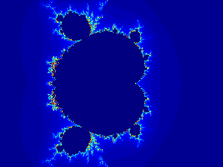
octave-3.0.1:1> Mc=mandelbrot(-2.1+1.05i,0.7-1.05i,640,64);
octave-3.0.1:2> imagesc(Mc)

Octave should then fire up Gnuplot and show a nice classic Mandelbrot set:

Classic Mandelbrot Set

Following this success, let's tackle the Julia set. The code should be very similar, with the exception that c should be a parameter of the function and z is the variable that needs initialisation using linspace and meshgrid. Furthermore, c doesn't need to be masked in the loop because it is a scalar value, not a matrix. So without further ado, here's the code for the ~octave/julia.m file:

julia.m

function M=julia(zmin,zmax,hpx,niter,c)
  vpx=round(hpx*abs(imag(zmax-zmin)/real(zmax-zmin)));
  [zRe,zIm]=meshgrid(linspace(real(zmin),real(zmax),hpx),
                     linspace(imag(zmin),imag(zmax),vpx));
  z=zRe+i*zIm;
  M=zeros(vpx,hpx);
  for s=1:niter
    mask=abs(z)<2;
    M(mask)=M(mask)+1;
    z(mask)=z(mask).^2+c;
  endfor
  M(mask)=0;
endfunction

Let's choose a value for c that corresponds to a point at the limit of convergence in the Mandelbrot set, such as -0.75+0.2i, and call the julia function:

octave-3.0.1:3> Jc1=julia(-1.6+1.2i,1.6-1.2i,640,64,-0.75+0.2i);
octave-3.0.1:4> imagesc(Jc1)

Octave should then refresh the Gnuplot windows and show the result:

Classic Julia Set for c=-0.75+0.2i

Classic Julia Set for c=-0.75+0.2i

Factorising Code

Considering both function are so similar, it should be possible to factorise code between them and have a core Mandelbrot/Julia function called by two simpler functions. The major difference is in the initialisation before the loop so can we factorise the loop? The only difference in the loop between the two functions is that in the mandelbrot function, c is masked because it is a matrix, whereas in the julia function, it is is not masked because it is a scalar. The solution is to transform c into a matrix of identical values in the julia function. We now have three files: mjcore.m that contains the core code and refactored mandelbrot.m and julia.m. Here is the full listing:

mjcore.m

function M=mjcore(z,c,niter)
  M=zeros(length(z(:,1)),length(z(1,:)));
  for s=1:niter
    mask=abs(z)<2;
    M(mask)=M(mask)+1;
    z(mask)=z(mask).^2+c(mask);
  endfor
  M(mask)=0;
endfunction

mandelbrot.m

function M=mandelbrot(cmin,cmax,hpx,niter)
  vpx=round(hpx*abs(imag(cmax-cmin)/real(cmax-cmin)));
  z=zeros(vpx,hpx);
  [cRe,cIm]=meshgrid(linspace(real(cmin),real(cmax),hpx),
                     linspace(imag(cmin),imag(cmax),vpx));
  c=cRe+i*cIm;
  M=mjcore(z,c,niter);
endfunction

julia.m

function M=julia(zmin,zmax,hpx,niter,c)
  vpx=round(hpx*abs(imag(zmax-zmin)/real(zmax-zmin)));
  [zRe,zIm]=meshgrid(linspace(real(zmin),real(zmax),hpx),
                     linspace(imag(zmin),imag(zmax),vpx));
  z=zRe+i*zIm;
  cc=zeros(vpx,hpx)+c;
  M=mjcore(z,cc,niter);
endfunction

Next

In the next article of this series, More on the Classic Sets, we wander around the Mandelbrot and Julia sets and see what happens to the Mandelbrot set when we choose a value for z0 that is different from 0. I also demonstrate how to save images to disk and talk about colour maps.