Making Noise with ImageMagick

The Case for Noise

At the @media conference earlier this year, Dan Rubin presented a talk entitled Designing Virtual Realism where he explained that we should try to reproduce real life textures when designing web sites to produce the feel bit in look & feel. If you are as useless with Photoshop or GIMP as I am, it is quite a difficult feat. However, Dan also had advice for visual design challenged people like me: if you do nothing else, at the very least, add noise. What he meant by that is to replace flat background colours with something that is not quite flat, adding subtle noise to the colour. As usual, ImageMagick is a great tool for that sort of things and gives you the opportunity to automate it.

Creating Noise

ImageMagick has an option to create random noise, which makes it very easy to start. Enter the following in a terminal window:

$ convert -size 100x100 xc: +noise Random noise.png

This will produce a PNG image 100 pixels wide by 100 pixels tall that will look something like this:

noise.png

Note that because the pixels in this image are completely random, it can be tiled, which is important if we want to use the final image as a tiled background.

Blurring the Noise

Next we need to blur the noise and desaturate it so that we can use it as a mask.

$ convert noise.png -virtual-pixel tile \
 -blur 0x1 -fx intensity -normalize noise-mask.png

Let's decompose this command to understand all the options:

-virtual-pixel tile

tells ImageMagick to use a tile of the picture for virtual pixels that are outside of the boundaries of the original. This is necessary because the blur algorithm uses neighbouring pixels to calculate a given colour. Using that option ensures that the result of the blur can also be used as a tile.

-blur 0x1

applies a fine blur to the image.

-fx intensity

selects the intensity channel only thus desaturating the image.

-normalize

stretches the contrast to ensure we go from pure black to pure white rather than average greys.

And here is the result:

noise-mask.png

Plain Colour Tiles

We then need two plain colour tiles that will be combined into the final image. Both colours should be very close to one another so that the noise is perceivable but not distracting. In this example, I will use two shades of red:

$ convert -size 100x100 xc:white -fill '#cc0000' -opaque white red1.png
$ convert -size 100x100 xc:white -fill '#bb0000' -opaque white red2.png

This is a rather weird syntax so let's explain it:

-size 100x100

creates an image that is 100x100 pixels.

xc:white

uses a pseudo-image that is completely white as a source image.

-fill '#cc0000'

selects the fill colour to be used by any following option, in this case a shade of red.

-opaque white

replaces all white pixels in the image (in this case the whole image) with the fill colour (red).

That's a bit convoluted but I haven't found a way to specify a hex colour value directly after xc:. If anybody knows better, please tell me.

Applying the Mask

The last step is to apply the mask created earlier to mix the two colour tiles:

$ convert red1.png red2.png noise-mask.png -composite red-noise.png

Et voilà! Some noise added to our plain red. And here is how the two compare, plain red on the left, noisy red on the right:

Plain Red vs Noisy Red

The difference is subtle but enough to give an impression of texture.

Script It

Last but not least, let's transform all of the above in a small shell script to be re-used later. Note that I am using bash here, which will work fine on Ubuntu or Mac OS-X but you may need to adapt it if you are using a different operating system:

noise.sh

#!/bin/bash

# Retrieve parameters and assign defaults if not found
size=${1:-50x50}
col1=${2:-#000000}
col2=${3:-#111111}
ofile=${4:-noise.png}

# Set the name of the temporary mask file
mask=/tmp/$$-mask.png

# Create temporary mask
convert -size $size xc: +noise Random -virtual-pixel tile\
        -blur 0x1 -fx intensity -normalize $mask

# Create both colours and compose with mask
convert -size $size xc:white -fill $col1 -opaque white\
        -size $size xc:white -fill $col2 -opaque white\
        $mask -composite $ofile
 
# Delete temporary file
rm $mask

To use it, you need to make it executable first:

$ chmod +x noise.sh

Then it's just a case of giving it a size, two colours and an output file name as parameters:

$ ./noise.sh 100x100 '#00cc00' '#00bb00' green-noise.png

Now, go make some noise and banish those boring plain backgrounds!

Fractals with Octave: Burning Ship

The story so far

• Classic Mandelbrot and Julia
• More on the Classic Sets
• Other Polynomials
• Trigonometric and Exponential Functions

After a long pause, here is the fifth instalment of this series on fractals with Octave. This time I will look at a fractal called the Burning Ship because of its output that looks like a ship going up in flames.

Burning Ship

The fractal is a Mandelbrot set that has a generating series defined by:

z_n+1=(|Re(z_n)|+i|Im(z_n)|)²+c

where the Re and Im are the functions that return the real and imaginary parts of a complex number. The initial condition is:

z₀=0

This fractal can be directly produced with the mandelbrot function we created in previous articles. In addition, we will take r=200 as a divergence limit.

octave-3.0.1:1> Mbs=mandelbrot(-2.5-2i,1.5+i,320,64,
> @(z,c) (abs(real(z))+i*abs(imag(z))).^2.+c,200);
octave-3.0.1:2> imagesc(Mbs)

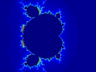
Octave should open the Gnuplot window and display an image similar to this:

Burning Ship

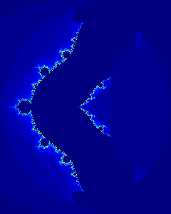
Now let's zoom on this fractal centre left by a factor of 30:

octave-3.0.1:1> Mbsz=mandelbrot(-1.8-0.06i,-1.7+0.02i,320,64,
> @(z,c) (abs(real(z))+i*abs(imag(z))).^2.+c,200);
octave-3.0.1:2> imagesc(Mbsz)

Octave should open the Gnuplot window and display an image similar to this:

Burning Ship, left centre zoom x30

As usual with a fractal like this, the zoomed image looks very similar to the original. Now let's have a look at a related fractal called the Bird of Prey.

Bird of Prey

In the same way that you can produce interesting variations on the classic Mandelbrot set by changing the power used in the series, we can do the same with the Burning Ship series. So let's increase the power in the series above from 2 to 3:

z_n+1=(|Re(z_n)|+i|Im(z_n)|)³+c

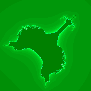
This cubic series produces a fractal called the Bird of Prey.

octave-3.0.1:1> Mbs3=mandelbrot(-1.5-1.5i,1.5+1.5i,320,64,
> @(z,c) (abs(real(z))+i*abs(imag(z))).^3.+c,200);
octave-3.0.1:2> imagesc(Mbs3)

You'll note that I chose the boundary values for the complex plane so that I would get a square image centered on the origin. Here is the resulting image:

Bird of Prey

Next

That's it for the Burning Ship. Next in this series, we will look at the original fractal that Gaston Julia was interested in.

Selective Colouring with ImageMagick

Following a recent Photojojo newsletter, I thought I would do some experimentation with black and white. But rather than use Photoshop or GIMP, I decided to use ImageMagick: the command line may seem like more effort at first but it gives more control and you can also put everything in a script for later re-use.

Choosing a good photograph

There are some photographs that come out great as black and white, others that don't. Generally, the best candidates are the ones that look a bit uninteresting in colour, generally because there isn't much colour in them to start with. It's easy to get that sort of shots in London: just go out on a cloudy day and you'll get likely candidates. And so, I shot this picture on Sunday afternoon while on the South Bank:

The Globe Theatre

Although the building is nice, the picture itself is quite dull: there is little colour in it apart from the red flags so it's an ideal candidate for black and white treatment.

Separating the channels

Following the Photojojo article, rather than transform that photograph into grey scale, I started by separating the red, green and blue channels, which is very easy to do with ImageMagick:

$ convert img.jpg -separate img_rgb_%d.jpg

Assuming your original image is called img.jpg, this will produce three images called img_rgb_0.jpg, img_rgb_1.jpg and img_rgb_2.jpg that correspond to the red, green and blue channels respectively:

Red, green and blue channels

The last one, the blue channel, is the best black and white in my opinion as it's got the strongest shadows and lightest sky. Having said that, the red flags in the original photograph were the main spots of bright colour and it would be interesting to bring them back in the black and white shot through selective colouring. So let's do that.

Creating a mask

To selectively colour the flags red in the black and white picture, I am going to combine the original shot with the blue channel image. For this, I need to create a mask that will tell ImageMagick what part of the original shot to use and what part of the blue channel image to use. For the mask, I need a black and white picture that is white where the flags are and black everywhere else: this way, I can tell ImageMagick to use pixels from the original image where the mask is white and pixels from the blue channel image where the mask is black.

Because the flags are red, the idea is to find all the pixels in the original image that are red and no other colour. We can do that by combining the three channel images. Pixels that are a shade of grey, anywhere between black and white will show as the same shade of grey on all three channels but pixels that are of a specific colour, such as red, will be of a light grey in their primary channel and very dark in the other two. Indeed, if you look at the three channel images, the flags show as very light in the red channel but nearly black in the other two. So to create our mask, we can subtract the green and blue channels from the red one.

First, let's subtract the green channel from the red one:

$ convert img_rgb_1.jpg img_rgb_0.jpg -compose minus \
 -composite img_rgb_0-1.jpg

Which produces the following image:

Green channel subtracted from the red one

We can already see the flags pop out of the picture but we can also still see the outline of the theatre. So let's subtract the blue channel from the image we just obtained:

$ convert img_rgb_2.jpg img_rgb_0-1.jpg -compose minus \
 -composite img_rgb_0-1-2.jpg

Green and blue channels subtracted from the red one

That looks good, except that the flags are now light grey rather than really white. It is still a good mask but as the grey pixels will mix both images we use, it will dilute the effect. To ensure that we have a full effect, we need to stretch the contract of the mask to have the background area really black and the flags area really white.

$ convert img_rgb_0-1-2.jpg -level 10%,30% img_mask.jpg

The values given after the -level option specify the percentage of white under which a pixel is considered black first followed by the percentage of white over which a pixel is considered white. There is no real perfect value for those so you need to experiment. In this example, the second value is quite low because we really want most grey pixels to be turned white for a sharp mask.

Stretched mask

You will note that there are some small dots of white at the bottom of the mask. That's slightly unexpected but we'll see in a minute what they are.

Creating the final picture

Now that we have a mask, we need to combine the blue channel image with the original image by applying the mask. This is the simplest use of the -composite operator:

$ convert img_rgb_2.jpg img.jpg img_mask.jpg \
 -composite img_final.jpg

This produces the final image. We can now see that the small dots of white at the bottom of the mask have let out some of the colour of the red flowers on the lamppost, which is a nice extra touch and which would have been forgotten had we created the mask by hand with a drawing tool. Such side effects are typical of such a tool that works on the whole image and can be welcome or not depending on the situation. In any way, it is always possible to tweak the mask manually in a drawing tool before applying it.

Final image

Bootnote

The photo in its original size is now visible on flickr.

Fractals with Octave: Trigonometric and Exponential Functions

The story so far

• Classic Mandelbrot and Julia
• More on the Classic Sets
• Other Polynomials

In this fourth instalment of this series on fractals with Octave, I'll have a look at the Mandelbrot and Julia sets generated by non-polynomial series. Polynomials are fine but they can be a bit boring so what about introducing a sine or exponential in the mix? The original idea for this came from an excellent set of articles and examples by Paul Bourke.

Sine function

The first series we will use is defined thus:

z_n+1=c sin(z_n)

That's simple enough and very easy to code in Octave so as our mandelbrot and julia functions now have the ability to take a generating series as argument, it should be no problem. But before doing that, we need to know what value to give to r so that we know when the series diverges and when we can stop iterating. In the very first article, we saw that:

[...] for a given polynomial series, there exists a value r such that if for any n, |z_n|>r, then the series diverges.

This only applies to polynomials. The series above is not a polynomial series and its condition for divergence is that the imaginary part of z_n be greater than 50. That doesn't work well with our current code that expects a simple integer. We could replace the integer parameter expected by the mandelbrot and julia functions with a function handle but that would make their usage more complex when using polynomial series. Luckily, we can have the best of both worlds because Octave uses a weakly typed language: the type of a parameter passed to a function is not specified in the function definition, meaning that you can pass anything, you just have to hope that it is what the function expects. While this can be seen as a drawback for long and complex programs where validation can be cumbersome, it is actually a useful feature for a high level language like Octave where functions tend to be short. To make it work, we need to modify the mjcore function so that it can accept a function handle or an integer as its fifth parameter and act accordingly. For this, we will use the Octave isa built-in function to identify whether the parameter is a function handle. Here's how to modify the mjcore function:

mjcore.m

function M=mjcore(z,c,niter,f,r)
  if(isa(r,"function_handle"))
    rf=r;
  else
    rf=@(z) abs(z)<r;
  endif
  M=zeros(length(z(:,1)),length(z(1,:)));
  for s=1:niter
    mask=abs(z)<rrf(z);
    M(mask)=M(mask)+1;
    z(mask)=f(z(mask),c(mask));
  endfor
  M(mask)=0;
endfunction

That's all great and now we should be able to create our first sine Mandelbrot. We need to make sure that we reverse the comparison operator in the last parameter because our code is built so that we provide a convergence condition rather than a divergence one:

octave-3.0.1:1> Msin=mandelbrot(-1.2*pi+0.9*pi*i,1.2*pi-0.9*pi*i,
> 320,64,
> @(z,c) c.*sin(z), @(z) abs(imag(z))<=50);
octave-3.0.1:2> imagesc(Msin)

And we end up with... a dark blue rectangle, not quite what was expected. This is because in this form, the value of z₀ is 0, therefore sin(z₀) is also 0 and so is c sin(z₀): the series is always null and never diverges. To correct this, we would need to have z₀=c, that is initialise the series to the values of c. But if we do that in the code of the mandelbrot function, it will break some of our previous examples. That is unless we can specify a special value of z₀ to the mandelbrot function to force it to initialise to z₀=c. A similar trick to what we did for r above can do that: if the given parameter is the special string "c", initialise to c, otherwise assume the parameter is an integer and initialise as before. Here is the modified mandelbrot function:

mandelbrot.m

function M=mandelbrot(cmin,cmax,hpx,niter,
                      f=@(z,c) z.^2.+c,r=2,
                      z0=0)
  vpx=round(hpx*abs(imag(cmax-cmin)/real(cmax-cmin)));
  z=zeros(vpx,hpx).+z0;
  [cRe,cIm]=meshgrid(linspace(real(cmin),real(cmax),hpx),
                     linspace(imag(cmin),imag(cmax),vpx));
  c=cRe+i*cIm;
  if(strcmp("c",z0))
    z=c;
  else
    z=zeros(vpx,hpx).+z0;
  endif
  M=mjcore(z,c,niter,f,r);
endfunction

After that modification, we can run the mandelbrot function again with our new special parameter:

octave-3.0.1:1> Msin=mandelbrot(-1.2*pi+0.9*pi*i,1.2*pi-0.9*pi*i,
> 320,64,
> @(z,c) c.*sin(z), @(z) abs(imag(z))<=50, "c");
octave-3.0.1:2> imagesc(Msin)

Octave should open the Gnuplot window and display an image similar to this:

Sine Mandelbrot Set

We can also generate a sine Julia set without any change to the julia function:

octave-3.0.1:1> Jsin=julia(-2.4*pi+1.8*pi*i,2.4*pi-1.8*pi*i,
> 320,64,1+0.5i,
> @(z,c) c.*sin(z), @(z) abs(imag(z))<=50);
octave-3.0.1:2> imagesc(Jsin)

Sine Julia Set

Cool stuff! So let's have a look at other non-polynomial functions and their output.

Cosine

This series is defined by:

z_n+1=i c cos(z_n)

And has the same convergence condition than the previous series.

octave-3.0.1:1> Mcos=mandelbrot(-1.2*pi+0.9*pi*i,1.2*pi-0.9*pi*i,
> 320,64,
> @(z,c) i.*c.*cos(z), @(z) abs(imag(z))<=50, "c");
octave-3.0.1:2> imagesc(Mcos)

Cosine Mandelbrot Set

octave-3.0.1:1> Jcos=julia(-2.4*pi+1.8*pi*i,2.4*pi-1.8*pi*i,
> 320,64,0.55+1.195i,
> @(z,c) i.*c.*cos(z), @(z) abs(imag(z))<=50);
octave-3.0.1:2> imagesc(Jcos)

Cosine Julia Set

Tangent

This series is defined by:

z_n+1=c tan(z_n)

And uses the same convergence function as a polynomial with the default value of r.

octave-3.0.1:1> Mtan=mandelbrot(-1.4+1.4i,1.4-1.4i,
> 320,64,
> @(z,c) c.*tan(z), :, "c");
octave-3.0.1:2> imagesc(Mtan)

Tangent Mandelbrot Set

octave-3.0.1:1> Jtan=julia(-1.4+1.4i,1.4-1.4i,
> 320,64,(1+i)*sqrt(2)/2,
> @(z,c) c.*tan(z));
octave-3.0.1:2> imagesc(Jtan)

Tangent Julia Set

Exponential

First, let's multiply the exponential using the following series:

z_n+1=c exp(z_n²)

This series uses the default values for r and z₀.

octave-3.0.1:1> Mexp1=mandelbrot(-1.4+2i,1.4-2i,
> 240,64,
> @(z,c) c.*exp(z.^2));
octave-3.0.1:2> imagesc(Mexp1)

Exponential Mandelbrot Set #1

Then, let's add to the exponential using the following series:

z_n+1=exp(z_n²)+c

This series also uses the default values for r and z₀.

octave-3.0.1:1> Mexp2=mandelbrot(-2.2+2i,1-2i,
> 240,64,
> @(z,c) exp(z.^2).+c);
octave-3.0.1:2> imagesc(Mexp2)

Exponential Mandelbrot Set #2

Cactus

Finally, let's draw a cactus using the following series:

z_n+1=z_n³+(z₀-1)z_n-z₀

This series uses the default values for r and the special value z₀=c.

octave-3.0.1:1> Mcactus=mandelbrot(-0.8+0.6i,0.8-0.6i,
> 320,64,
> @(z,c) z.^3.+(c.-1).*z.-c,:,"c");
octave-3.0.1:2> imagesc(Mcactus)

Cactus Mandelbrot Set

Next

Next in this series, we will look at a fractal called the Burning Ship.

Lloyds TSB phishing scam

I just received an email which claims to come from Lloyds TSB. As I am not a customer of the bank, it is obviously a scam. I've been looking on the bank's web site in an attempt to report it to them but there doesn't seem to be any email address advertised where you can do so. There are a couple of telephone numbers for their customers but that's it. Surely, it would be useful to them to have copies of those emails, if only to know they exist and to warn their customers. But it seems they are not interested. Maybe it's a good thing I don't bank with them then.

Photos from Peru

I came back from Peru a week ago and spent a good part of last week tweaking and cleaning the best of them. They are now visible on flickr. The tweaking and cleaning I do on photos is very simple and consists in:

• stretching the contrast if required;
• removing fluff and dirt mark left on the lens or the sensor;
• very occasionally, cropping the shot.

So no heavy Photoshop (or in that instance GIMP) processing, just the bare minimum.

It's all relative

I'm in Peru. We just spent a couple of days around the Cañon de Colca, one of the deepest canyons in the world. The place where we stayed last night, Chivay, is at 3700 metres above sea level and on the way there we stopped at a viewpoint that was 4900 metres above sea level, higher than Mont Blanc. The area around Chivay and the canyon is lush and green and if it wasn't for the thin air, you'd easily forget that you are at an altitude that is higher than most of the Alps' ski resorts.

Nobody told the locals either, as explained by one of the girls in the group this morning: she asked the landlady of the hotel where she stayed overnight whether she kept llamas or alpacas, to which the landlady replied "we don't do that here, only in the mountains". That'd be the steep bits above 4000 metres that we see in the distance then.

Bootnote

This was written on the bus between Chivay and Puno yesterday and uploaded today.

ExifTool on Ubuntu

A while ago, I blogged about installing ExifTool on Ubuntu. There's actually a much simpler way to do this. ExifTool is part of the standard packages directly available from the Ubuntu repositories so it can be installed in one line using apt-get, no need for that make malarkey I mentioned last time:

$ sudo apt-get install libimage-exiftool-perl

Et voilà, ExifTool installed and ready to go!

Making Skype work with PulseAudio in Ubuntu Intrepid and Jaunty

Following my sound issues with Skype on Ubuntu, I did a bit more research and eventually found an excellent how-to article on PulseAudio in the Ubuntu forums. Appendix C explains how to get Skype to work properly and indeed it is a doodle and means there is no need to kill PulseAudio when using Skype! I've tested it in Intrepid and Jaunty and it works a treat. To quote the article, here's how to do it:

Open Skype's Options, then go to Sound Devices. You need to set "Sound Out" and "Ringing" to the "pulse" device, and set "Sound In" to the hardware definition of your microphone. For example, my laptop's microphone is defined as "plughw:I82801DBICH4,0".

You will have to experiment with the different options for "Sound In" until you find the correct one: choose an option, click on "Make a test call" until you find the option that works. On my machine, here's what the option window looks like:

Skype Options, Sound Devices Tab

Google Street View

Like a number of people, I was a bit dubious about Google Street View. If you want to see what a place looks like, there are enough photographs on the web for you to find, why would you want to go look at bad photographs taken by a passing car? However, where Street View does come into its own is when coupled with driving directions in Google Maps: for each intersection, you can have a picture of what it looks like with an arrow that tells you where to go. This is a fantastic visual aid when going to a place you are not familiar with.

Driving directions with Street View

Adding a Static Address to the DHCP Server

I've got a Lexmark X9575 all-in-one printer. Up to now, it was connected to the Mac via USB. I wanted to reconfigure it to connect it to the network instead so that I can use it with other computers. But I wanted to do so in such a way that it would get its network configuration via DHCP while keeping a fixed address and be resolvable via DNS.

The first thing I did was to remove the printer setup from the Mac (no, you can't change the configuration, you have to un-install and re-install, thank you Lexmark!). Then I connected the printer to the network switch with a standard RJ45 cable. It requested a DHCP lease form the server immediately and the DNS entries got updated. That was a good start. However, the IP address was part of the dynamic range and therefore unpredictable and the name of the printer was hard-coded to the very non-intuitive ET0020002C5B7A. I wanted something more memorable like lexmark-printer.

To force a fixed IP address is quite simple, as explained in this DHCP mini-howto. I just added the following to the /etc/dhcp3/dhcpd.conf file:

host lexmark-printer {
 hardware ethernet 00:20:00:2c:5b:7a;
 fixed-address 192.168.1.250;
}

Restarted the DHCP server:

$ sudo /etc/init.d/dhcp3-server restart

And it didn't work, for two reasons:

• The DHCP server already had a lease assigned so wasn't going to renew it;
• The printer already has an IP address configured so wasn't going to renew it either.

To solve the first problem, I needed to force the expiry of the lease on the DHCP server. The ISC DHCP server stores leases between restarts in a file called /var/lib/dhcp3/dhcpd.leases. So revoking the lease can be done by updating that file, removing the entry for the given lease and restarting the DHCP server.

The second problem was of the same ilk: go to the printer's TCP/IP configuration, set DHCP to no, save the settings, go back into them, set DHCP back to yes and that forced the printer to request a new lease.

That gave me a static address for the printer while still keeping it managed by DHCP. However, in such a case, the DHCP server doesn't update the DNS database. This has to be done manually, by adding the following in the forward lookup file:

lexmark-printer.home.   IN A    192.168.1.250

And this in the reverse lookup file:

250.1.168.192.in-addr.arpa. IN PTR  lexmark-printer.home.

Then of course, a restart of the DNS server is required:

$ sudo /etc/init.d/bind9 restart

Skype Sound Issues

Skype is not available in the Ubuntu repositories but you can get hold of it (and a few other things) through medibuntu. However, it looks like that version of Skype has a problem with sound on Ubuntu 8.10 Intrepid Ibex, as detailed in this bug report. The workaround suggested in the discussion that consists in killing pulseaudio before launching Skype works for me so that's good news. Even better news, it looks like the problem is fully sorted in Ubuntu 9.04, which is currently in beta. So, until then, I will use the workaround.

One lesson to learn from this though, is that if you ever have a problem with a piece of software on Linux, a good practice is to start that software from the command line: the output in the terminal window is invaluable for developers and maintainers to understand the problem and is a good place to start in order to find a solution to it. Quite often, just putting the error message in Google will return a number of articles and bug reports on that exact problem.

Upgrading the Server from Gutsy to Hardy

My silent server that provides DNS, DHCP, Subversion and other services to my home network hadn't been upgraded since it was first installed and had been running Ubuntu 7.10 (aka Gutsy Gibbon) quite happily all this time. But with 7.10 reaching end of life in a few weeks, I felt it was time to upgrade and that today was the day to do so.

The first port of call is the upgrade notes and in particular the Hardy note to upgrade from 7.10 to 8.04. Make sure you read the "Before You Start" section at the beginning of that note before you start. So taking this into account, here is the sequence of what I did for that upgrade:

Refresh the package index

It's always good to do that once in a while and especially before an upgrade.

$ sudo apt-get update

Update all packages

Before an upgrade, it's essential to ensure that you are on the latest version of packages for your current release.

$ sudo apt-get upgrade

You will likely need to reboot after that, especially if the upgrade includes a new kernel. If in doubt, reboot anyway.

$ sudo init 6

Install update-manager-core

That's the bit that will perform the upgrade so you need to make sure it's there. If in doubt, install it, apt-get will tell you if you already have the latest version.

$ sudo apt-get install update-manager-core

Upgrade!

That's the biggie that will take a long time and may ask you some questions in the process. If you ever get any question, make sure you read them carefully. Defaults tend to be sensible so it shouldn't wreck your system but that doesn't excuse you from being sensible and paying attention.

$ sudo do-release-upgrade

A few things to note on the upgrade process:

• I was doing my upgrade through SSH. If things go wrong, you can potentially lose connection with your server and it can all end in tears so the upgrade process warns you about this and starts a second SSH daemon on a different port (9004 in my case but it will tell you). I had no problem installing over ssh but be careful nonetheless.
• If you have a DHCP server configured, as I do, it will probably notify you that the file /etc/dhcp3/dhcpd.conf file has been modified on your server and ask you whether you want to replace it with the new one it just downloaded or keep the old one. You need to keep the old one if you want your settings to be preserved. To be on the safe side, make a copy of it just in case.
• Because of a well documented bug in Debian upon which Ubuntu is based, the upgrade process will re-generate any SSL key, in particular the RSA keys used by SSH. That will affect us later and I'll explain what to do about it.

Once the upgrade is finished, the script will ask you of you want to reboot immediately. Unless you have a good reason to reboot manually, you can let the upgrade process do that for you.

Updating the SSH keys on the client machine

If you attempt to reconnect to your server via ssh straight after the upgrade, you will be greeted by a worrying message and you won't be able to go further:

Helsinki:~ brunogirin$ ssh bruno@szczecin
@@@@@@@@@@@@@@@@@@@@@@@@@@@@@@@@@@@@@@@@@@@@@@@@@@@@@@@@@@@
@    WARNING: REMOTE HOST IDENTIFICATION HAS CHANGED!     @
@@@@@@@@@@@@@@@@@@@@@@@@@@@@@@@@@@@@@@@@@@@@@@@@@@@@@@@@@@@
IT IS POSSIBLE THAT SOMEONE IS DOING SOMETHING NASTY!
Someone could be eavesdropping on you right now (man-in-the-middle attack)!
It is also possible that the RSA host key has just been changed.
The fingerprint for the RSA key sent by the remote host is
dc:11:1a:78:f4:34:c3:a2:ab:9d:52:1e:98:6d:7f:36.
Please contact your system administrator.
Add correct host key in /Users/brunogirin/.ssh/known_hosts to get rid of this message.
Offending key in /Users/brunogirin/.ssh/known_hosts:2
RSA host key for szczecin has changed and you have requested strict checking.
Host key verification failed.

This is normal and is due to the fact that the upgrade process has re-generated the ssh RSA keys on the server. Those keys are stored on all client machines that have previously connected to that server so that they can verify the identity of the server. To resolve that problem, the error message is giving us a hint. On the example above taken from my OS-X box, it tells me that the offending key is on line 2 of file /Users/brunogirin/.ssl/known_hosts. So open that file in an editor and remove the offending line then try to connect again. As it doesn't have the key anymore, it will ask for confirmation before adding the new one to that file and let you connect:

Helsinki:~ brunogirin$ ssh bruno@szczecin.home
The authenticity of host 'szczecin.home (192.168.1.253)' can't be established.
RSA key fingerprint is dc:11:1a:78:f4:34:c3:a2:ab:9d:52:1e:98:6d:7f:36.
Are you sure you want to continue connecting (yes/no)? yes
Warning: Permanently added 'szczecin.home' (RSA) to the list of known hosts.

Note that if you have several keys for the same host, for instance if you've connected through its name and IP address in the past, it may give you another warning, as shown on my Ubuntu laptop:

Warning: the RSA host key for 'szczecin' differs from the key
 for the IP address '192.168.1.253'
Offending key for IP in /home/bruno/.ssh/known_hosts:1
Are you sure you want to connect (yes/no)?

Once again, it tells you which is the offending key so you can remove it and attempt to connect via the IP address to renew the key. Note that this only works as explained above if SSH on the client is configured so that the StrictHostKeyChecking option is set to ask. If it is set to no, it will never check and will happily connect. If it is set to yes, you will have to update the keys manually. See man ssh_config for the full details.

There you go: apart from the SSH malarkey at the end, it was rather straightforward and very quick too! In fact, it took me more time to write this post that do the upgrade.

Bootnote

Now that I have this server on 8.04, I could upgrade immediately to 8.10 but I'll leave that for another day. In fact, considering that 8.04 is an LTS release, I may leave my server on that version until the next LTS release, 9.10 aka Karmic Koala, scheduled for October.

Custom Page Numbering with LaTeX

I'm currently doing a home course on short story writing. Or should I say I attempt to as I haven't been returning my assignments very promptly. Anyway, one of the requirements is that each assignment is formatted in such a way that the footer of each page contains the page number, starting at 1 on the first page, and the letters mf for More Follows on every page except the last one. In order to do this, I need to be able to set a specific footer for the last page and one for all other pages. I tried to do that with OpenOffice.org to start with but there was no way to identify whether you were on the last page using a macro with version 2.4, which is what I was using when I started. As you would expect, it is surprisingly easy to do with LaTeX, provided you import the correct packages.

• In order to specify a custom footer (or header), I will need the fancyhdr package;
• I will also need to be able to use some if/then/else logic to output something different whether I am on the last page or not, this is provided by the ifthen package;
• Finally, I will need to know whether I am on the last page, which is provided by the aptly named lastpage package.

Putting all this together, the document's code needs to do the following:

• Import all relevant packages;
• Set the page style to fancy;
• Set all headers and footers to blank;
• Set the header and footer lines to 0 points (optional, you may like the defaults);
• Set the right hand side footer so that it implements this logic:
  • If the page is the last one, print nothing;
  • Otherwise, print mf.
• Set the left hand side footer to the current page's number.

And here is the resulting code:

\documentclass[a4paper,12pt]{article}
\usepackage{lastpage}
\usepackage{ifthen}
\usepackage{fancyhdr}

\pagestyle{fancy}
\fancyhf{}
\renewcommand{\headrulewidth}{0pt}
\renewcommand{\footrulewidth}{0pt}
\fancyfoot[R]{\ifthenelse{\thepage=\pageref{LastPage}}{}{mf}}
\fancyfoot[L]{Page~\thepage}

\begin{document}

The content of the document goes here.

\end{document}

Updated Cow Analogy

I just received the following by email:

After the recent teetering-on-the-edge-of-total-economic-and-financial-meltdown couple of weeks it seems economic systems and their workings have pushed their way into the need-to-know-category. Well, we can now simplify this all by explaining 9 economic models with cows.

Socialism

You have 2 cows.

You give one to your neighbour.

Communism

You have 2 cows.

The State takes both and gives you some milk.

Fascism

You have 2 cows.

The State takes both and sells you some milk.

Nazism

You have 2 cows.

The State takes both and shoots you.

Bureaucratism

You have 2 cows.

The State takes both, shoots one, milks the other, and then throws the milk away...

Traditional Capitalism

You have 2 cows.

You sell one and buy a bull.

Your herd multiplies, and the economy grows.

You sell them and retire on the income.

An American Corporation

You have 2 cows.

You sell one, and force the other to produce the milk of four cows.

Later, you hire a consultant to analyse why the cow has dropped dead.

2008 Venture Capitalism

You have 2 cows.

You sell three of them to your publicly listed company, using letters of credit opened by your brother-in-law at the bank, then execute a debt/equity swap with an associated general offer so that you get all four cows back, with a tax exemption for five cows. The milk rights of the six cows are transferred via an intermediary to a Cayman Island Company secretly owned by the majority shareholder who sells the rights to all seven cows back to your listed company. The annual report says the company owns eight cows, with an option on one more. You sell one cow to buy a new president of the United States, leaving you with nine cows. No balance sheet provided with the release. The public then buys your bull.

Fractals with Octave: Other Polynomials

The story so far

• Classic Mandelbrot and Julia
• More on the Classic Sets

In the third instalment of this series on fractals with Octave, I want to change the polynomial series used to generate the Mandelbrot and Julia sets. So far, I've used the classic series, defined by:

z_n+1=z_n²+c

In the previous articles, I showed what happened when you varied the initial values for z₀ and c but why not go further and use a different polynomial altogether?

Code review

Before jumping into the thick of it, let's have a look at the code produced so far. We created 4 functions:

function M=mjcore(z,c,niter)

The core function shared by the mandelbrot and julia functions;

function M=mandelbrot(cmin,cmax,hpx,niter)

The function that produces a colour map image as per the Mandelbrot algorithm;

function M=mandelbrotz0(cmin,cmax,hpx,niter,z0)

A variation of the mandelbrot function that takes an extra argument in order to specify an initial z₀ value;

function M=julia(zmin,zmax,hpx,niter,c)

The function that produces a colour map image as per the Julia algorithm.

There is very little difference between the mandelbrot and mandelbrotz0 functions: mandelbrot just uses a default value of 0 for z0. In fact, we could merge both functions into one using the default argument construct supported by Octave. Here's a new version of the mandelbrot.m file that uses it:

mandelbrot.m

function M=mandelbrot(cmin,cmax,hpx,niter,z0=0)
  vpx=round(hpx*abs(imag(cmax-cmin)/real(cmax-cmin)));
  z=zeros(vpx,hpx).+z0;
  [cRe,cIm]=meshgrid(linspace(real(cmin),real(cmax),hpx),
                     linspace(imag(cmin),imag(cmax),vpx));
  c=cRe+i*cIm;
  M=mjcore(z,c,niter);
endfunction

Having done this, we can now create the classic Mandelbrot image as we did previously, using four arguments:

octave-3.0.1:1> Mc=mandelbrot(-2.1+1.05i,0.7-1.05i,640,64);

Create the Mandelbrot image with z₀=0.2+0.2i by adding a fifth argument:

octave-3.0.1:2> Mz0=mandelbrot(-2.1+1.05i,0.7-1.05i,640,64,0.2+0.2i);

And we can delete the mandelbrotz0.m file. Note that you could also explicitly tell Octave to use the default for the fifth argument by specifying a colon (:) in its place, so you could produce the classic Mandelbrot this way:

octave-3.0.1:3> Mc=mandelbrot(-2.1+1.05i,0.7-1.05i,640,64,:);

This is not very useful in this context but we will see a use for it later.

Function handles and anonymous functions

In order to be able to change the polynomial used to calculate the fractal image, we need to be able to specify to the mjcore function what function to use when calculating the series. We could create a whole library of mjcore derivatives but that would quickly get tedious. Instead, we can use Octave's function handles. A function handle is a fancy way to say that in Octave, any variable can be a function. Therefore, we can just pass the function as an argument of the mjcore function. And while we're at it, we'll also pass r as an argument because, as we saw in the first article, the value for r is dependant on the function used in the series. So here is a modified version of that function:

mjcore.m

function M=mjcore(z,c,niter,f,r)
  M=zeros(length(z(:,1)),length(z(1,:)));
  for s=1:niter
    mask=abs(z)<r;
    M(mask)=M(mask)+1;
    z(mask)=f(z(mask),c(mask));
  endfor
  M(mask)=0;
endfunction

That's all good and well but we've just moved the problem further into the mandelbrot and julia functions: those functions will have to specify parameters accordingly and use sensible defaults so that if we omit the values for f and r, it will calculate the classic sets using the series z_n+1=z_n²+c (i.e. the function f=z²+c) and r=2. To do that, we are going to use the default argument construct explained above and combine it with an anonymous function. Using anonymous functions, we can define a variable f that is a handle on a function that implements the classic algorithm:

octave-3.0.1:4> f=@(z,c) z.^2.+c;

As shown above, we can use exactly the same syntax to specify default arguments to the mandelbrot and julia functions. Here are the new versions of those two functions:

mandelbrot.m

function M=mandelbrot(cmin,cmax,hpx,niter,
                      f=@(z,c) z.^2.+c,r=2,
                      z0=0)
  vpx=round(hpx*abs(imag(cmax-cmin)/real(cmax-cmin)));
  z=zeros(vpx,hpx).+z0;
  [cRe,cIm]=meshgrid(linspace(real(cmin),real(cmax),hpx),
                     linspace(imag(cmin),imag(cmax),vpx));
  c=cRe+i*cIm;
  M=mjcore(z,c,niter,f,r);
endfunction

julia.m

function M=julia(zmin,zmax,hpx,niter,c,
                 f=@(z,c) z.^2.+c,r=2
                 )
  vpx=round(hpx*abs(imag(zmax-zmin)/real(zmax-zmin)));
  [zRe,zIm]=meshgrid(linspace(real(zmin),real(zmax),hpx),
                     linspace(imag(zmin),imag(zmax),vpx));
  z=zRe+i*zIm;
  cc=zeros(vpx,hpx)+c;
  M=mjcore(z,cc,niter,f,r);
endfunction

Cubic sets

We can now produce cubic Mandelbrot and Julia sets by setting the power to 3 instead of 2:

octave-3.0.1:5> Mn3=mandelbrot(-1.2+1.6i,1.2-1.6i,240,64,
> @(z,c) z.^3.+c);
octave-3.0.1:6> imagesc(Mn3)

Cubic Mandelbrot Set

octave-3.0.1:7> Jn3=julia(-1.6+1.2i,1.6-1.2i,320,64,0.4,
> @(z,c) z.^3.+c);
octave-3.0.1:8> imagesc(Jn3)

Cubic Julia Set for c=0.4

Quartic sets

Increasing the power to 4, we get quartic sets:

octave-3.0.1:9> Mn4=mandelbrot(-1.2+1.6i,1.2-1.6i,320,64,
> @(z,c) z.^4.+c);
octave-3.0.1:10> imagesc(Mn4)

Quartic Mandelbrot Set

octave-3.0.1:11> Jn4=julia(-1.6+1.2i,1.6-1.2i,320,64,-1,
> @(z,c) z.^4.+c);
octave-3.0.1:12> imagesc(Jn4)

Quartic Julia Set for c=-1

Note that for a series defined by the equation z_n+1=z_n^p+c, the resulting Mandelbrot set will show p-1 secondary "blobs" while the Julia set will show p secondary "blobs".

Decimal power

The power doesn't have to be an integer. Using a decimal value, such as 2.5, generates the following Mandelbrot image, that is halfway between the normal and cubic sets:

octave-3.0.1:13> Mn2_5=mandelbrot(-1.6+1.2i,1.6-1.2i,320,64,
> @(z,c) z.^2.5.+c);
octave-3.0.1:14> imagesc(Mn2_5)

Mandelbrot Set for p=2.5

Complex power

Using a complex power, such as 2+0.1i, generates a skewed set:

octave-3.0.1:15> Mn2_01i=mandelbrot(-2.2+1.2i,1.0-1.2i,320,64,
> @(z,c) z.^(2+.1i).+c);
octave-3.0.1:16> imagesc(Mn2_01i)

Mandelbrot Set for p=2+0.1i

More complex polynomial

Using a series based on a more complex polynomial, such as z_n+1=z_n²+z_n+c, generates the following set:

octave-3.0.1:17> Mp=mandelbrot(-2+1.05i,0.8-1.05i,320,64,
> @(z,c) z.^2.+z.+c);
octave-3.0.1:18> imagesc(Mp)

Mandelbrot Set for series z_n+1=z_n²+z_n+c

Bootnote

Having modified the mandelbrot function to include the f and r arguments before the z0 argument, we now need to use the colon argument for f and r to produce a classic Mandelbrot with a different value of z0:

octave-3.0.1:2> Mz0=mandelbrot(-2.1+1.05i,0.7-1.05i,640,64,:,:,0.2+0.2i);

I could have left the z0 argument in fifth position to avoid having to do this but I felt that the f and r arguments were more likely to be provided so are better specified first in the function's signature.

Next

In the next article in this series, Trigonometric and Exponential Functions, we'll look at non-polynomial series.

Fractals with Octave: More on the Classic Sets

The story so far

• Classic Mandelbrot and Julia

In the second instalment of this series on fractals with Octave, I will generate more images by changing some of the parameters of the different functions presented in the first article. But before doing that, I'll briefly explain how to save the generated images and say a word on colour maps.

Saving images

The images that the functions described in the previous post generate are colour mapped images. Each element of a result matrix is an integer value that corresponds to a colour index. Octave has a very easy way to save that type of images using the well named saveimage function. To save the images generated, we just need to do:

octave:1> saveimage(file name, matrix, type, colour map);

The file name parameter is the name of the image file we want to save the image to. Give it a .ppm extension, we'll see why in a second. The matrix parameter is the matrix generated by the mandelbrot or julia functions presented in the previous article. The type parameter is the type of the image: we will use the PPM type as it is supported natively by Octave so that attribute should just be ppm. The colour map attribute is a colour map to use in the file. Octave has a default colour map that contains 64 colours from dark blue to light blue, then from yellow to red and white, similar to a contour map. It can be invoked by the colormap command. Putting all this together, creating a classic Mandelbrot image and saving it can be done this way:

octave:1> M=mandelbrot(-2.1+1.05i,0.7-1.05i,320,64);
octave:2> saveimage("mandelbrot.ppm", M, "ppm", colormap);

The PPM file format is understood natively by Linux but if you want to transform it into a more widely used format such as GIF or PNG, you can use ImageMagick or The GIMP. Avoid the JPEG format as it's not well suited to that type of computer generated images.

That's all well and good but what if you want your generated images to use a different colour map from the default? Let's create one. Octave understands a colour as a row vector that has 3 elements corresponding to the red, green and blue components of a colour. Each element is a real value between 0.0 and 1.0. So for example bright red would be [1, 0, 0] and 50% grey would be [0.5, 0.5, 0.5]. A colour map is a 3 column matrix where each row in the column is a colour. As an example, the following is a 5 colour map that defines a gradient from bright red to bright green:

   1.00000   0.00000   0.00000
   0.75000   0.25000   0.00000
   0.50000   0.50000   0.00000
   0.25000   0.75000   0.00000
   0.00000   1.00000   0.00000

We can build such a gradient by using the linspace command to evenly spread values. We will need to do that for each red, green and blue component and then combine all three with the cat command. Each vector produced by linspace will represent a column in the colour map matrix. However linspace produces row vectors so we need to transpose them before concatenating them using the ' operator. The following will produce a 64 value gradient from dark blue to white:

mycolmap=cat(2,
linspace(0, 1, 64)',
linspace(0, 1, 64)',
linspace(0.2, 1, 64)'
);

The resulting colour map can then be used to save the image. Note that for best results, the number of colours in the colour map should be the same as the number of iterations used when producing the fractal image.

Zooming into the Mandelbrot set

With the preamble out of the way, let's create some more fractal images. You can now save them for posterity! Some great images can be obtained by zooming somewhere on the edges of the Mandelbrot set. Let's zoom to the top centre of the set:

octave:1> Mcz=mandelbrot(-0.27+i,0.05+0.76i,320,64);
octave:1> imagesc(Mcz)

Octave should open the Gnuplot window and display the following image:

Mandelbrot Set, Top Centre Zoom

This image shows a number of artefacts that are similar to the complete set. Zooming further on those would show them in more details. And as this is a fractal set, you can zoom as much as you want and discover more interesting structures.

Mandelbrot with a non-null z₀

In the first article, we built the mandelbrot function based on the assumption that the initial value of the z_n series, z₀, was 0 for all values of c. It doesn't have to be. So let's create a modified mandelbrot function that can set a different value for z₀ and call it mandelbrotz0. Copy the mandebrot.m file described in the previous article into a mandelbrotz0.m and modify it accordingly:

mandelbrotz0.m

function M=mandelbrotz0(cmin,cmax,hpx,niter,z0)
  vpx=round(hpx*abs(imag(cmax-cmin)/real(cmax-cmin)));
  z=zeros(vpx,hpx).+z0;
  [cRe,cIm]=meshgrid(linspace(real(cmin),real(cmax),hpx),
                     linspace(imag(cmin),imag(cmax),vpx));
  c=cRe+i*cIm;
  M=mjcore(z,c,niter);
endfunction

Then, let's run this function with z₀=0.2+0.2i:

octave:1> Mz0=mandelbrotz0(-2.1+1.05i,0.7-1.05i,320,64,0.2+0.2i);
octave:2> imagesc(Mz0)

Octave should refresh the Gnuplot window and display the following image:

Mandelbrot Set, z₀=0.2+0.2i

Quirky! It's as if the Mandelbrot set was exploding like a ruptured balloon! Other values produce interesting results and the further they are from 0, the more distorted the set is.

Zooming into the Julia set

After the experiments with the Mandelbrot set above, let's explore the Julia set a bit more than we did last time, using c=-0.1+0.9i. Let's calculate the whole set for this value:

octave:1> Jc2=julia(-1.6+1.2i,1.6-1.2i,320,64,-0.1+0.9i);
octave:2> imagesc(Jc2)

Which produces the following image:

Julia Set, c=-0.1+0.9i

Then, let's zoom 10 times to a point slightly off centre:

octave:1> Jc2z=julia(-0.16+0.24i,0.16,320,64,-0.1+0.9i);
octave:2> imagesc(Jc2z)

Julia Set, c=-0.1+0.9i, zoom x10

And again:

octave:1> Jc2zz=julia(-0.016+0.072i,0.016+0.048i,320,64,-0.1+0.9i);
octave:2> imagesc(Jc2zz)

Julia Set, c=-0.1+0.9i, zoom x100

Cool pictures, don't you think?

Bootnote

Having created a slightly more generic mandelbrotz0 function above, we can now re-write and simplify the original mandelbrot function by calling mandelbrotz0:

mandelbrot.m

function M=mandelbrot(cmin,cmax,hpx,niter)
  M=mandelbrotz0(cmin,cmax,hpx,niter,0);
endfunction

Next

In the next article of this series, Other Polynomials, we look at what happens when we use a different complex series than the standard one.

Using the LaTeX letter document class

LaTeX offers a variety of built-in document classes. One of them is letter, which is designed for writing official letters, such as the one I just did to the (inept) agency that manages my flat. However, that standard document class is not very well liked: it's the ugly little duckling of the LaTeX document classes. But when you just have to get things done, better the devil you know than the one you don't. So here's a quick summary of easy tweaks I applied to my letter to bend the default document class to my needs.

Structure

The letter document class requires a specific structure. It is designed so that you can write several letters to several recipients while using the same return address. The basic structure of a letter document looks something like this:

Basic structure of a letter document

\documentclass{letter}

\address{The return address}
\signature{Your signature}

\begin{document}
\begin{letter}{The recipient's address}

\opening{The opening, such as: Dear Sir,}

The body of the letter

\closing{The closing, such as: Best regards,}

\end{letter}
\end{document}

The letter environment that is enclosed in the document environment looks superfluous at first. The idea is that you can have several letter environments when you want to produce more than a single letter: this can be very useful for mailings.

Top space

The document class introduces a lot of white space at the top. This is good for a multi-page letter but looks really awkward on a single page letter. So, I did what the TeX FAQ suggests and added the following in the preamble, just after the \documentclass command:

Preamble to remove the initial top space

\makeatletter
\let\@texttop\relax
\makeatother

\begin{document}

Adding a reference

As my managing agent specified a reference in the letter they sent me, I wanted to include that reference in my letter, just after their address but with some small vertical space in between. There is no obvious way to do that so I just added it to the end of the recipient's address with a space of length \parskip:

Adding a reference

\begin{letter}{The recipient's address\\[\parskip]
Your ref: The reference}

Adding some vertical space before the closing sentence

The closing sentence is printed very close to the last paragraph in the letter. I wanted a bit more space so added the following just before the \closing command:

Adding space before closing

\vspace{3\parskip}
\closing{The closing, such as: Best regards,}

Adding space between the closing and the signature

When writing a letter, I like leaving enough space between the closing sentence and the printed signature so that I can add a hand written signature once it's printed. The standard space is too small for this. However, considering both lines are printed by the \closing command, there is no obvious way to include any space in between. However, looking at the letter.cls code, it appears that the standard template adds 6 times the \medskipamount length in between the two lines so the simple way to change that space is to change the relevant length just before the \closing command:

Adding between the closing and signature

\vspace{3\parskip}
\addtolength{\medskipamount}{2\medskipamount}
\closing{The closing, such as: Best regards,}

This will multiply the \medskipamount length by 3 and as result multiply the space between closing and signature by 3 as well. This works great for a single letter but will not have the intended result when you have multiple letters in the same document. The way to avoid this is to save the original length and restore it afterwards:

Adding between the closing and signature

\vspace{3\parskip}
\setlength{\oldmedskipamount}{\medskipamount}
\addtolength{\medskipamount}{2\medskipamount}
\closing{The closing, such as: Best regards,}
\setlength{\medskipamount}{\oldmedskipamount}

With those few tricks, I got a letter that was close enough to what I wanted. I could probably have spent a lot more time tweaking it or trying alternative document classes but this particular job didn't warrant me spending too much time on it.

Designing Good Error Handling

Usability is an important subject in software design. Your application can be the coolest thing since sliced bread, if it's difficult to use, people will just not bother. We all know that. There are lots of books and articles on usability. However, such material often forgets about one important aspect of usability: error handling and messages. When your application encounters an error, whether it is due to something the user did or to a bug, it is extremely important to ensure it behaves in a way that makes sense to the user, even more important than for normal behaviour. This is because when an error occurs, your user will typically be stopped in his tracks and asked to resolve a problem he wasn't expecting to be faced with. If the error handling adds to the confusion rather than help, the user will not know what to do and his confidence about the application and his own ability to understand it will significantly diminish. So here are a couple of example of what not to do, helpfully provided over the past week by applications I use at work.

Cryptic error message

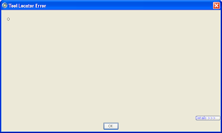
We use Borland StarTeam at work to manage change and configuration. When starting the application earlier this week, I was faced with the following error message:

Yes, the error message consists of a single zero. Difficult to do any shorter or any more cryptic. At that point, I am given two options: a Details button and an OK one. Assuming the Details button may lead me to a more understable explanation, I clicked it and it showed me the following message:

This is absolutely meaningless for anybody who is not a Java developer. And even for those who are, it doesn't really help, it only shows that there is a bug in the product where an internal array is not checked for size before accessing its first entry. It doesn't tell me whether the application will keep working or whether it will horribly crash when I click OK. It so happens that clicking OK made the message box disappear and the application kept working normally after that.

So, how can we improve on such a message? The best way in my opinion would be to display a message to the user explaining that an internal problem has occurred in the application and how they can report it to Borland. What is displayed in the details screen would be invaluable to the developers in order to correct the bug. So directions on how to send that information to the product team would make the user feel that the company cares about the qulity of their product and that they are ready to receive bug reports. Not all users would actually go through the steps of reporting the bug but some would.

Lack of information

Another error I was faced with this week came from the automated backup tool. This tool, which is installed on all laptops will continually backup changes in the user's folder to a central server. It runs in the background, is relatively unobtrusive and flexible enough that you can select sub-directories that you don't want to have backed up. However, it sometimes require your attention and will pop up a message. I was faced with this one yesterday:

Contrary to the previous example, this message is in plain English and I can understand every word of it. However, it is worded in such a generic way that I have no idea whether I should click OK or Cancel. I don't know what part-completed actions it refers to and therefore don't know whether those actions should be completed or not. I suspect that they should because the default button is the OK one but I can't be sure. Also note that the word scan is misleading: it only makes sense to me because I have a fair idea of how the backup tool works but it could make the user think this is a message from the anti-virus system.

So, what could be done to make it more useful? First, the message should identify what application triggered it. It is important in this case because it is triggered by a background process and is completely unrelated to what the user was doing at the time. Then the obvious thing to do would be to detail what actions are pending and require attention. However, this may not be enough. If the actions' descriptions are too cryptic, that won't help the user make a decision. So the message should also ensure that the descriptions for the pending actions are clear and concise.

Conclusion

Usability is good but it should also go hand in hand with error handling. So next time you design a piece of software, make sure all the error messages that can potentially be displayed to the user are clear and include enough information, especially if the user is expected to take a decision based on the message. If the message is triggered by an unexpected error, consider giving the user a way to report the error so that you can correct the bug in a subsequent version.